Quick start: a 5-minute tour
This walks through a complete, real example — comparing two BCL2L1 isoforms in top-down mode, adding a phosphorylation, and searching for confounding proteins — using nothing but the app's own built-in Ensembl lookup. No files to prepare.
1. Lock in the global settings
At the top of the page, two panels apply to every input path: MS strategy (top-down vs. middle-down, and the usable mass range) and MS resolution parameters (the instrument model and fragmentation scoring mode).
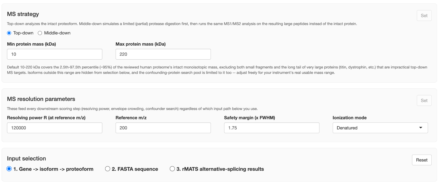
Leave the defaults for this tour (Top-down, 10–220 kDa, R = 120,000 @ m/z 200, Calibrated scoring) and click both Set buttons. This isn't cosmetic — every button below (Load isoforms, Run sequence analysis, Run analysis) stays disabled until both are set at least once. See MS strategy and MS resolution parameters for what each field actually controls.
2. Load a gene's isoforms
Under Input selection, Option 1 ("Gene → isoform → proteoform") is selected by default. Type a gene symbol and click Load isoforms:
BCL2L1
This fetches every protein-coding transcript for the gene from the precomputed exon index, plus a real translated sequence for each from Ensembl (cached to disk after the first fetch). BCL2L1's 40 transcripts collapse to 9 distinct protein sequences.
3. Check two isoforms and add a PTM
Open the Isoform catalog (collapsed by default after the first load) and check two rows —
say ENST00000941693 (251 aa) and ENST00000925014 (250 aa). Each row has its
own PTM spec box; type a modification directly:
14_S_Phospho
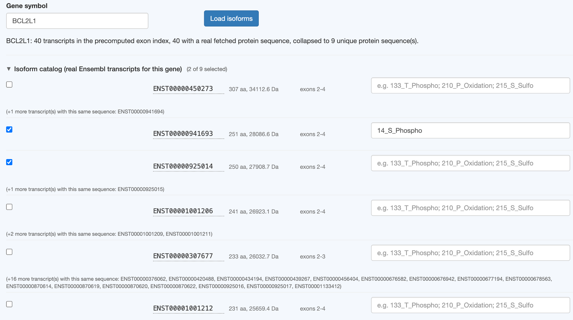
That's <1-based residue>_<amino acid>_<Unimod name> — see
PTM specification syntax for the full grammar, multi-PTM
combinations, and what happens when a spec doesn't match the sequence. Every valid PTM group
becomes its own extra row in the proteoform table below, alongside the unmodified form — it
doesn't replace it.
4. Review the proteoform table and run the analysis
Scroll down. The Result proteoform table lists every checked isoform plus every valid PTM combination, each with its own computed mass. Pick one as the confounder-search target, then click Run analysis.
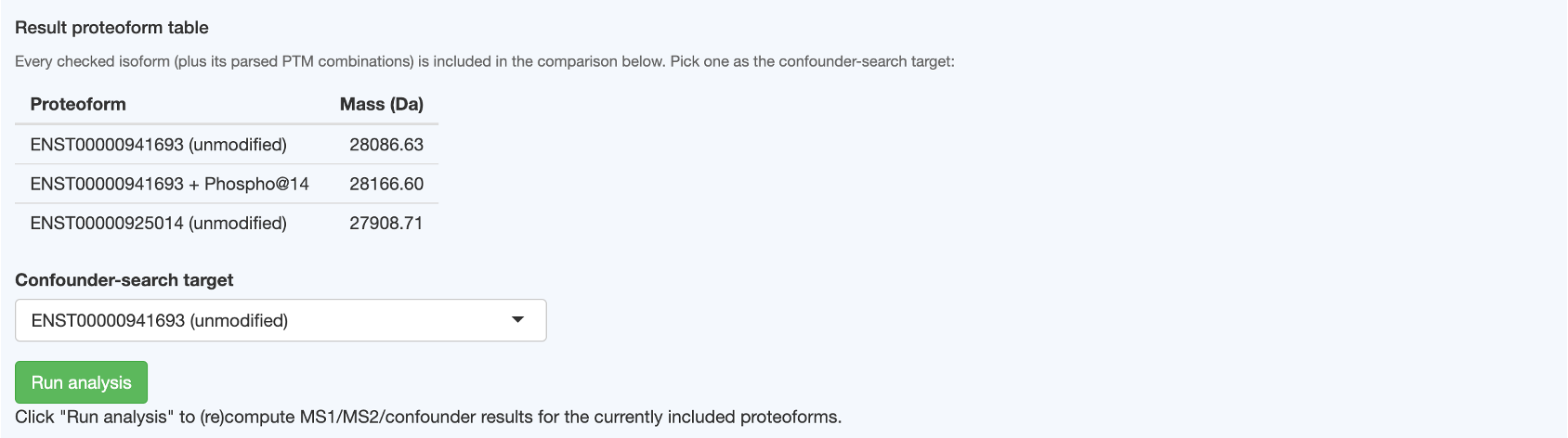
Notice the PTM row: ENST00000941693 + Phospho@14 at 28166.60 Da, +79.97 Da over the unmodified
28086.63 Da — exactly Unimod's phospho mass delta.
Analysis runs in two visible stages (watch the progress toast): first the MS1/MS2 comparison for everything checked, then a search for confounding proteins (cheap — no isotope computation yet).
5. Read the relevant-proteoform comparison
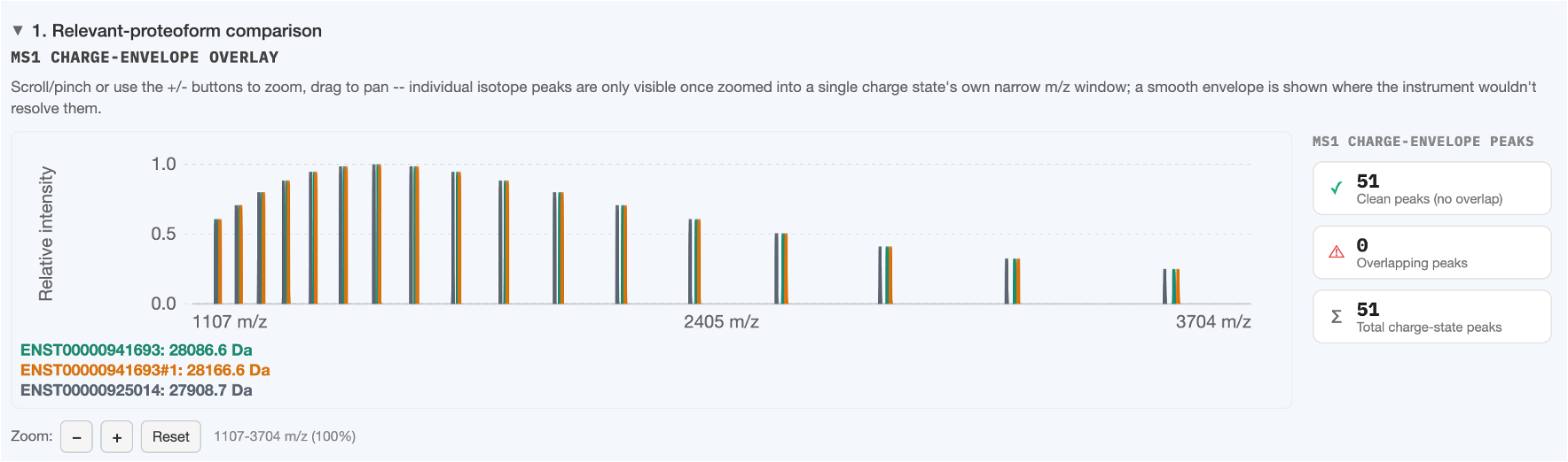
Section 1 shows the MS1 charge-envelope overlay for all three checked proteoforms side by side, with an aggregate stats panel (how many of their charge-state peaks are cleanly separable):
Below it, the MS2 fragment ladder — one row per proteoform, aligned on a shared exon axis, with live unique/partial/common counts next to each title:
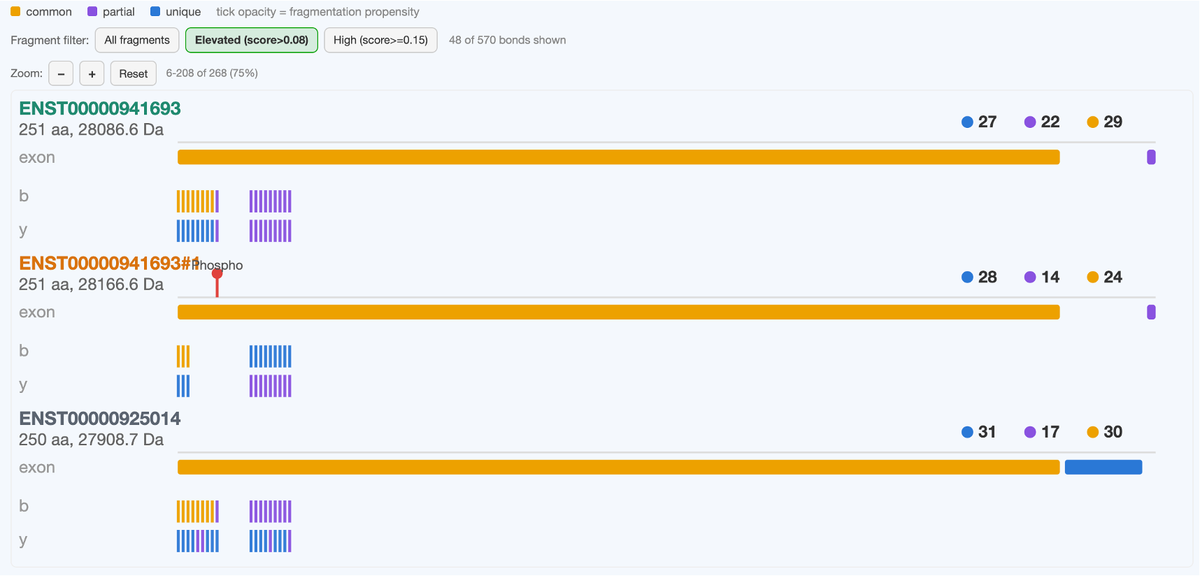
The red "Phospho" marker on the second row shows exactly where the modification sits. See Section 1: Relevant-proteoform comparison for how to read the colors, zoom into individual isotope peaks, and inspect one fragment ion's own isotope pattern.
6. Select which confounders to compare
Section 2 doesn't jump straight to a chart — it first shows you every real candidate the search found (capped at the 30 highest-priority, since a target can realistically collide with hundreds), with a checkbox per row so you can rule candidates out using outside evidence (e.g. an RNA-seq expression call):
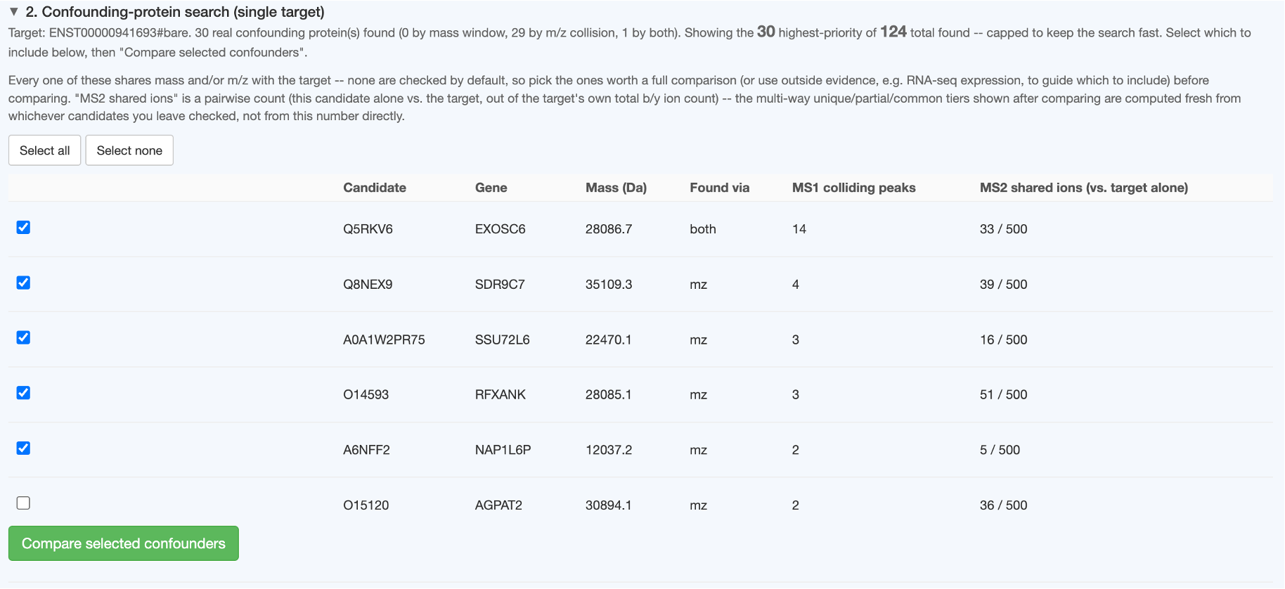
Leave everything checked (or deselect what you know isn't expressed) and click Compare selected confounders. See Section 2: Confounding-protein search for what "found via mass/m-z/both" means and how the MS2 shared-ion count is computed.
7. Read the confounder comparison
Once the (isotope-pattern-heavy) comparison finishes, you get the same two chart types as Section 1 — but here the target is drawn in green, on top, and every confounder gets its own color:
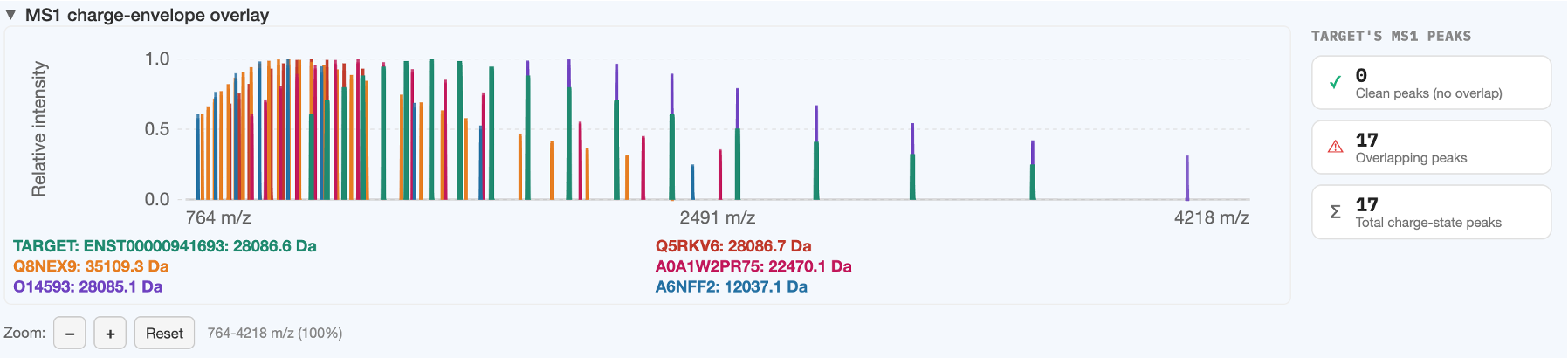
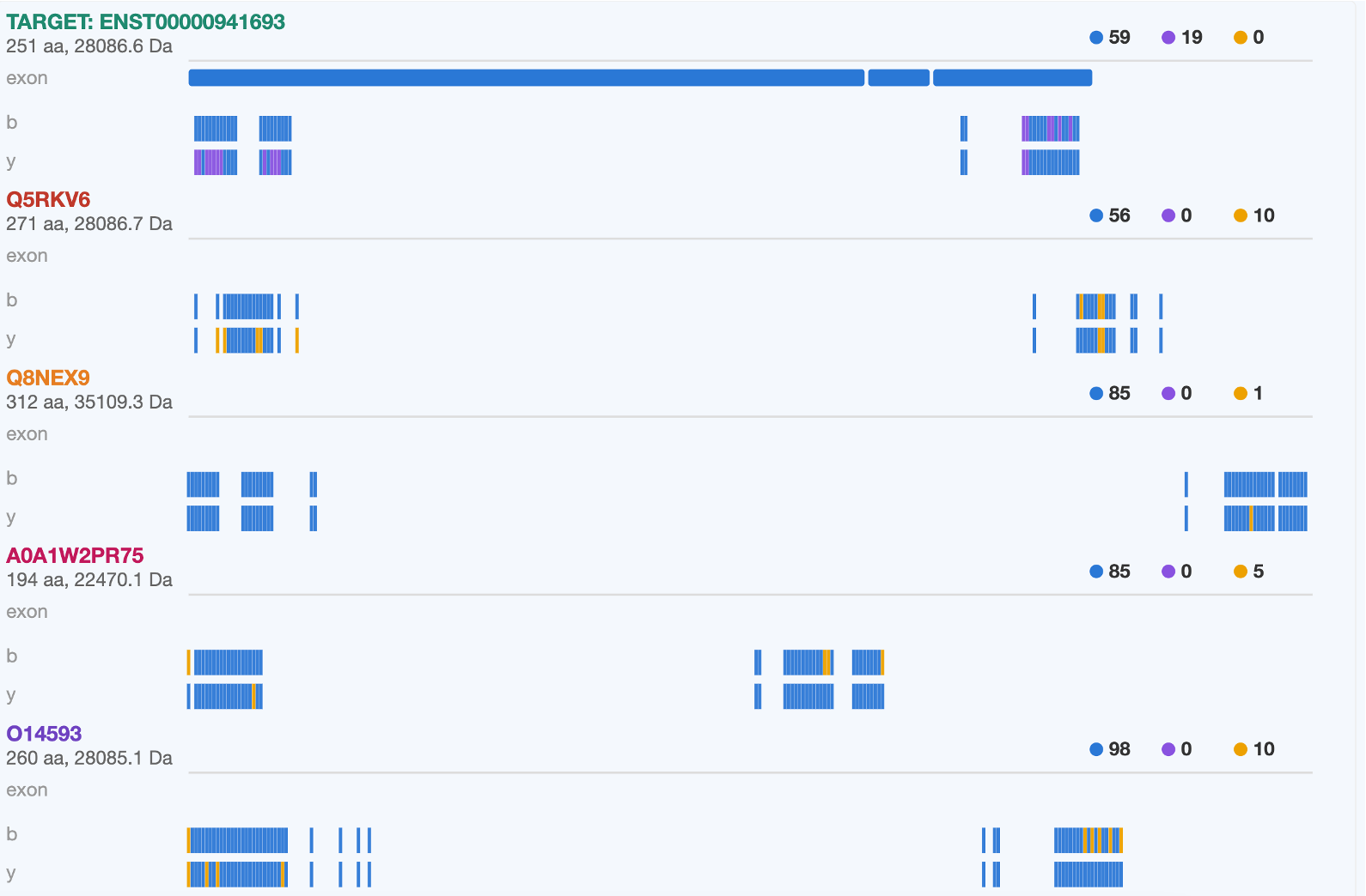
That's the full loop: load → check → (optionally modify) → run → read MS1/MS2 → select and compare confounders. From here, see:
- Middle-down mode if your workflow digests first
- Option 2: FASTA sequence / Option 3: rMATS for the other two input paths
- Interacting with the charts for zoom/pan/hover/click details