Section 2: Confounding-protein search

Searches the full reference human proteome for real proteins — from any gene — that could be confused with your chosen confounder-search target (picked from the proteoform table before clicking Run analysis). See Relevant vs. confounding proteins for the concepts behind this search; this page covers the actual on-screen workflow.

This section runs as two separate steps, deliberately: search first, then an explicit choice about which results to spend the expensive computation on.

Step 1: the search (automatic, fast)

Runs immediately as part of Run analysis — no isotope-pattern computation yet, just a mass/m-z index lookup and a lightweight per-candidate fragment-ladder comparison. Produces the status line and candidate table:

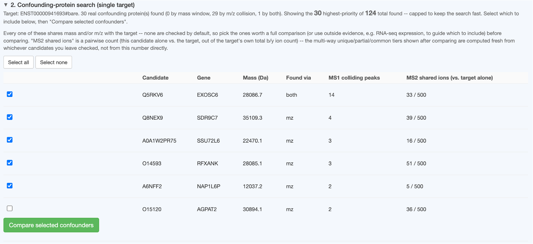
The status line reports how many were found by mass window, by m/z collision, and by both — with the shown vs. total-found counts highlighted in bold when the list is capped (see why the list is capped).

Table columns:

Column	Meaning
Candidate	UniProt accession
Gene	Gene symbol (parsed from the reference proteome's UniProt headers; blank for the rare entry with no GN= field)
Mass (Da)	Candidate's own intact mass
Found via	mass, mz, or both — see Relevant vs. confounding proteins
MS1 colliding peaks	How many distinct target charge-state peaks this candidate's envelope lands on
MS2 shared ions (vs. target alone)	Cheap pairwise fragment-mass overlap — this candidate alone vs. the target

Step 2: choosing what to compare

Every row is checked by default. Deselect any candidate you have outside evidence for excluding — most commonly, an RNA-seq expression call telling you it isn't actually expressed in your sample. Select all / Select none speed up bulk changes. Click Compare selected confounders to run the full comparison on whatever's still checked.

This second step is genuinely more expensive than the search — it computes a real isotope-pattern MS1 envelope for every selected confounder plus the target, which is the same per-candidate cost that made an uncapped, unfiltered candidate list impractically slow in earlier versions of this tool. Narrowing your selection here directly controls how long this step takes.

The comparison results

Once it finishes, you get the same two chart types as Section 1 — MS1 overlay and MS2 ladder — but for the target against your chosen confounders:

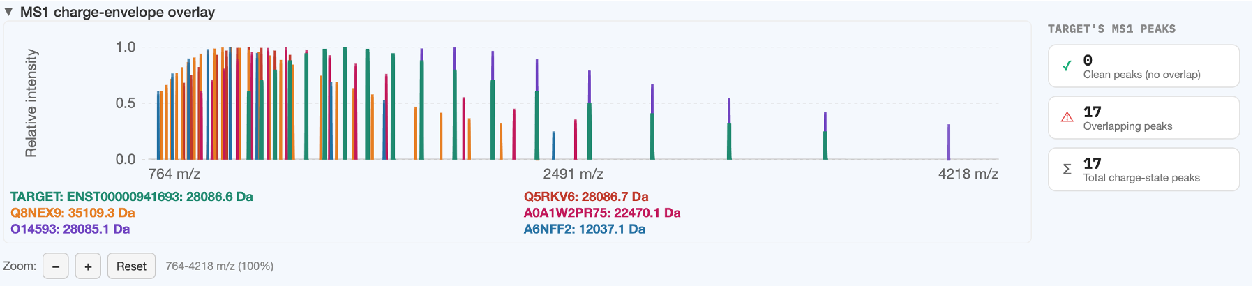
The target's curve is always drawn last (on top), thicker and fully opaque, specifically because m/z-domain confounders are curated to share peaks with the target — without this, a target curve can get visually buried under a dozen confounder curves at exactly the positions that matter most. Each confounder gets its own color from a fixed palette, cycling if you have more confounders selected than palette colors.

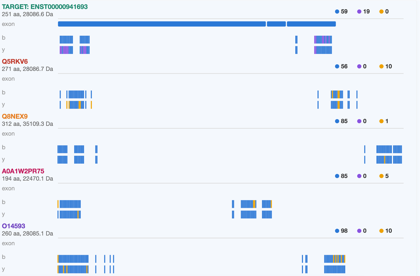
The MS2 ladder here shows only the target's own row, tiered against whichever confounders you selected — deselect a confounder and re-compare to see which of the target's fragments become "unique" once that specific confounder is out of the picture (see Tier colors).

Re-running with a different selection

Change checkboxes and click Compare selected confounders again at any time — this re-runs only the compare step, reusing the same search results, so it's faster than a fresh Run analysis. Clicking Run analysis itself always re-runs the search from scratch and resets your selection.